

THE CHALLENGE OF MODELLING CATASTROPHE EVENTS
The very last painting by Salvador Dali was titled The Swallow’s Tail – Serieson Catastrophes. Dali was greatly interested in the catastrophe theory developed
by the French mathematician René Thom, and referred to it as “the
most beautiful aesthetic theory in the world”. Thom’s catastrophe theory
describes how small changes in parameters of a stable nonlinear system can
lead to a loss of equilibrium and dramatic, on the level of catastrophic,
change in the state of the system.
Thom described equilibrium topological
surfaces and corresponding discontinuities that exist under certain conditions.
An equilibrium state is associated with the minimum of its potential
function; according to the catastrophe theory, a phase transition or a discontinuity
can be associated with only a limited number of stable geometric
structures categorising degenerate critical points of the potential function.
The Swallow’s Tail includes two of the so-called elementary catastrophes
taken directly from Thom’s graphs: the swallowtail and cusp geometries.
Dali was captivated by the catastrophe theory, especially after he met Thom.
Topological Abduction of Europe – Homage to René Thom, an earlier painting by
Dali, even reproduces in its bottom left corner the formula describing the
swallowtail elementary catastrophe geometry.
There have been numerous attempts to apply the catastrophe theory to
describing and predicting physical events. Returning from art to science, we
are faced with the challenge of assessing the frequency and severity of
natural and man made catastrophes that can lead to massive insurance
losses. The challenge is daunting, and developing a model to accomplish
this goal is a very practical task – with no surrealistic elements, even if the
results of catastrophes can often appear surreal.
This article introduces important concepts in modelling catastrophic events for the purpose of
analysing insurance risk securitisation. Issues examined here provide an
understanding of why modelling catastrophe risk is essential and why it is often so challenging.
Predicting the unpredictable
events and their impact on insured losses is within a probabilistic framework.
Catastrophe modelling has evolved in recent decades: its role in
quantifying insurance risk is critical and credible. The credibility of the
modelling tools continues to grow as they incorporate more and more of the
latest scientific research on catastrophic events and the insurance-specific
data that determines the impact of the catastrophes on insurance losses.
IMPORTANCE OF CATASTROPHE MODELLING TO INVESTORS
Wherever the payout on insurance-linked securities is tied to the possibleoccurrence of insured catastrophe losses, catastrophe modelling is the most
important tool for investors in analysing the risk of the securities and determining
the price at which they would be willing to assume this risk.
Superior ability to model insurance risk of catastrophic events is a source
of competitive advantage to investors in securities linked to such risk. This
ability can serve as an important differentiator and an indispensable tool in
a market that remains inefficient and suffers from the problem of asymmetric
information and general information deficiency.
The chapter on catastrophe bonds provided a brief overview of the structure
of the models used in analysing the insurance risk of property
catastrophe securitisations; it also examined important outputs such as
exceedance curves that specify probabilities of exceeding various loss levels.
It is equally important to understand inputs to the models.
The seemingly straightforward task of understanding the results, such as
interpreting the risk analysis included in the offering documents for cat
bonds, is actually the most important and the most challenging. If the
modelling software is a complete black box to an investor, any analysis of its
output is limited and deficient.
Not understanding the modelling tools also detracts from the usefulness of the sensitivity analysis that might be included in the offering documents; it makes it difficult to make any adjustments to improve on what is included in the documents.
It is unrealistic for most investors to become familiar with the inner
workings of catastrophe modelling software to get a better insight into
the risk involved in insurance-linked securities. The cost–benefit analysis
does not justify developing such expertise in house. Only true specialists
can afford this luxury. However, it is beneficial to any investor in catastrophe
insurance-linked securities to be familiar with the basic methodology of modelling catastrophe risk. This, at the very least, will allow investors to interpret the data in the offering circulars on a more sophisticated
level.
MODELLING CATASTROPHE INSURANCE RISK OF INSURANCE-LINKED SECURITIES
The article on catastrophe bonds provided an overview of the moderncatastrophe modelling technology and described the main modules of a
catastrophe modelling software provided by the three recognised independent
providers of insurance catastrophe modelling services, AIR
Worldwide, EQECAT and Risk Management Solutions (RMS). The chapter
also introduced concepts such as exceedance probability curve and return
period, and included a summary of sensitivity analysis and stress testing
that can be performed in evaluating insurance-linked securities.
The output of a catastrophe model is based on thousands or even millions
of years of simulated natural events and their financial impact on a given
insurance portfolio. This output can then be used to determine the probability
distribution of cashflows for a catastrophe bond or another security
linked to the risk of catastrophic events.
In fact, the modern models are not limited to natural catastrophes: models
of manmade catastrophes have also been developed. For example, terrorism
models have been developed to model the risk of catastrophe losses
resulting from such acts.
In this article, more information on the practical ways to model the
cat risk of ILS is added, along with a description of the available modelling
tools, their benefits and their limitations. First, however, the basics of
the science of natural catastrophes are described, since they form the framework
for the generation of catastrophe scenarios used by these software
tools.
THE SCIENCE OF CATASTROPHES
It is neither possible nor necessary for an investor to have in-house expertson the actual science underlying catastrophe models; basic understanding,
however, at the very least allows us to ask the right questions and to bring
a degree of transparency to the black-box view of the models.
Seismology is the study of earthquakes and the physical processes that
lead to and result from them. In the broader sense, it is the study of earth
movement and the earth itself through the analysis of seismic waves.
Earthquake prediction per se is not possible, but it is possible to identify
probabilities of earthquakes of specific magnitude by geographic region; in

as well.
Climatology and meteorology are the study of weather and atmospheric
conditions, with the latter focused on the short-term analysis of weather
systems and the former on the long-term analysis of weather patterns and
atmospheric phenomena.
The study of catastrophic weather events such as
hurricanes is a specialised branch of this science. In recent years, significant
progress has been made in understanding the dynamics of weather-related
catastrophes, and in assessing both long-term and short-term probabilities
of such events.
Structural engineering and several related fields permit the analysis of
damage to physical structures given the occurrence of a specific natural catastrophe.
This analysis is important for assessing insurance losses that can
result from a catastrophe such as hurricane or earthquake.
Epidemiology and medicine offer yet another example of study of catastrophes,
examining pandemic-type catastrophe events and their impact on
the population.
Manmade catastrophes are as difficult to predict as those caused by
nature; disciplines ranging from structural engineering to political science
can provide input into creating a probabilistic model of this type of catastrophic
events.
EARTHQUAKE FREQUENCY AND SEVERITY
A simple relationship between earthquake frequency and magnitude isdescribed by the Gutenberg–Richter law. It states that, for a given long
period of time in a certain region, the number N of earthquakes of magnitude
M or greater follows the power law
N(M) = 10a–bM,
which can alternatively be written as log N(M) = a – bM, where a and b are
constant. b usually, but not always, falls in the range between 0.8 and 1.2.
This relationship, specifying that an earthquake magnitude has a left-truncated
exponential distribution, holds surprisingly well for many territories
and earthquake magnitudes.
It can be used to obtain rough estimates of the
probability of earthquakes, even of magnitudes not observed, based on the
observations of earthquakes of other levels of magnitude.
Another important relationship is the Omori–Utsu law,1 which describes
the aftershock frequency of an earthquake. According to the Omori–Utsu
law, the rate of aftershocks decays after the main shock as
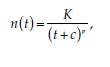
c, and p are constant. The c constant is the time-offset parameter describing
the deviation from the power law immediately after the main shock. The
Gutenberg–Richter law can be used to describe the distribution of aftershocks
by magnitude, which shows that the aftershock magnitude decay
can also be described by a power law.
The Reasenberg–Jones model combines the Guttenberg–Richter and Omori–Utsu laws to describe the intensity both of the main shock of an earthquake and its aftershocks.

According to Bath’s Law, in an earthquake, the difference in magnitude
between the main shock and its strongest aftershock is constant and independent
of the earthquake magnitude. All of these models should be
considered in a probabilistic framework.
It is important to note that the scientific definition of aftershocks,
according to which they can happen years or decades after the main shock,
differs from the insurance definition, which has a very narrow time range
for what constitutes an earthquake event.
Insurance-linked securities such as catastrophe bonds follow the same narrow definition of an earthquake, with aftershocks having to fall within a defined short period of time after the
main shock; otherwise, an aftershock might be considered a separate earthquake
event, and in that case it might have different coverage terms, it might
not be covered at all, or it might trigger second-event coverage.
The basic phenomenological laws such as the Gutenberg–Richter and

suggest. However, such simple laws are obviously insufficient for modelling
earthquakes, and several more sophisticated models have evolved for
this purpose.
EARTHQUAKE LOCATION
The vast majority of earthquakes occur on tectonic plate boundaries; thoughsome, typically smaller ones, do occur within the plates. Earthquakes within
the tectonic plates usually happen in the zones of fault or weakness, and
occur only in response to pressure on the plate originating from its
boundary.
The three categories of tectonic plate boundaries are spreading
zones, transform faults and subduction zones, each of which can generate its
own type of earthquake. Most spreading zones and subduction zones are in
the ocean, while transform faults can occur anywhere and are among the
best studied.
A global map of tectonic plates is presented in Figure 4.3, overleaf; it
shows the main tectonic plates and the boundary lines between them.
The hypocentre, where a rupture happens, is typically not very deep
under the earth’s surface for transform faults. In other words, the distance
between the hypocentre and the epicentre is relatively small.
Compressional and dilatational movements tend to follow straight patterns, at least for
“simple” earthquakes such as those that involve limited changes to the original
earthquake slip. The study of faults plays a major part in determining
the probability distributions of earthquakes in different areas.

levels that have a certain probability of occurring. Figure 4.4, opposite,
shows the US national seismic hazard map that displays shaking levels,
expressed as peak ground acceleration (PGA), at the probability level of 2%
over the period of 50 years. Other maps developed by the US Geological
Survey (USGS) correspond to the 5% and 10% probability of exceedance
over the 50-year period. The map shown was developed in 2008; the USGS
produces a fully revised version of the national seismic hazard maps
approximately once every six years.
The national seismic hazard maps are
important in insurance catastrophe modelling even if the modellers disagree
with the methodology used in developing the maps: the maps form the basis
for many building codes, which in turn determine the level of property
damage in case of an earthquake of a certain magnitude.
The two main types of earthquake models are fault- and seismicity-based.
The fault-based models rely on fault mapping; each known fault or fault
segment has a statistical function associated with the recurrence time for
earthquakes of specific magnitude.
In the simplest case, it is assumed that following an earthquake at a fault, stress on the fault has to be “renewed” by the tectonic processes until the next earthquake occurs. This view, while
fully stochastic, implies a certain degree of regularity of earthquakes that

models are also referred to as renewal models. Poisson, Weibull, gamma or
lognormal distributions can be used in modelling time between earthquakes,
even though other arrival process distributions are sometimes
utilised as well.
The Poisson renewal process, with an exponential distribution
of recurrence times, is the simplest but probably least accurate. In its
simplest form the Poisson fault-based model is time-independent. In
contrast to the fault-based models, seismicity-based models assume that
observed seismicity is the main indicator of the probability of future earthquakes.
The use of the Gutenberg–Richter law or a similar relationship then
allows the observed frequency of small earthquakes to be used for estimating
earthquakes of greater magnitude.
This approach does not require
information on the faults or even knowledge of their existence; it overcomes
a drawback of fault-based models, which can fail because many faults are
not yet mapped correctly, and some are not mapped at all. Seismicity-based
models are also called cluster models: the occurrence of several smaller
earthquakes might signify the coming of a bigger one.
Renewal processes can be used also for describing clustering events. Aftershock models allow
us to project past seismicity forward to arrive at a time-dependent proba-bility distribution of earthquakes at a specific location. The fault- and seismicity-
based models are not mutually exclusive: elements of both are
employed in modelling, in particular for the better-researched faults for
which there is also more extensive seismicity data available.
Some parts of the world have high levels of earthquake-related insurance
risk. They combine greater probability of earthquakes, due to being situated
on or close to a fault line, and the concentration of insured risk exposure. All
of Japan and part of California are examples of such high-risk areas.
Japan is located in a very seismically active area and has very high density
of population and insured property. Earthquakes in Japan have claimed
many lives and caused significant property damage.
The growth in population and property has led to the situation whereby a repeat of one of the
historically recorded earthquakes would now result in enormous losses.
Estimates of the overall (not only the insured) cost of a repeat of the great
1855 Ansei-Edo earthquake today go as high as US$1.5 trillion.
Tokyo sits at the junction of three tectonic plates: it is located on the Eurasian plate; while
not far from the city the Pacific tectonic plate “subducts” from the east, and
the Philippine Sea tectonic plate “subducts” from the south. Of particular
concern is the plane fragment under the Kanto basin, detached from either
the Pacific or the Philippine Sea tectonic plate, whose position could lead to
a large-magnitude earthquake in the already seismically active region.
Japanese earthquakes have been modelled very extensively, but there
remains a significant level of uncertainty as to the probability distribution of
their frequency and severity.
This particularly high level of uncertainty has
to be taken into account in any analysis of earthquake risk in Japan.
It has been said that the occurrence of a large-magnitude earthquake in a
densely populated area in California is a question of not if but when. The
San Andreas Fault is situated where the North American tectonic plate and
the Pacific tectonic plate meet, with the North American plate moving southward and the Pacific plate northward. The fault, shown on the next figure goes almost straight through San Francisco, with the city being on the North American plate, slightly to the east of the San Andreas Fault.
Los Angeles is also situated dangerously close to the fault line, but is located
to the west of it on the Pacific tectonic plate. San Andreas is a transform
fault; transform faults tend to produce shallow earthquakes with the focus
close to the surface.
A number of studies have concluded that there is a high probability of a
major earthquake at the San Andreas fault system, in particular in its
southern part, where stress levels appear to be growing and where there has

the southern part of the fault has a higher probability of a major earthquake
is not universally accepted. There is an agreement that all areas along the
fault, including San Francisco, which experienced a major earthquake in
1906, are at significant risk.
MORE ON EARTHQUAKE MODELLING
A numerical simulation approach has been used for modelling earthquakeparameters. The nature of the earthquake phenomenon and its inherent
uncertainty invites the probabilistic approach, and simulation is the natural
way to implement it. Models have been developed for describing ground
motion, stresses at the faults, fault dimensions, rupture velocities and many
other parameters.
The sheer number of unknowns and random variables involved in simulating
earthquakes leads to attempts to simplify the problem by focusing on
only major factors affecting the development of earthquakes, and by using
phenomenological laws in place of direct simulation for some variables. The
results have been mixed.
While every one of the existing models and
approaches is incomplete, relies on many simplifying assumptions and
could be easily criticised, there has not yet emerged a way to adequately
simulate such complex natural phenomena as tectonic developments and
earthquakes.

Even though the numerical simulation approach is generally the best to
portray the behaviour of complex systems, incorrectly specifying some of
the variables or the interdependences among the variables can lead to incorrect
results. Even simpler approaches, by necessity neglecting interdependence
of some of the variables involved, are very challenging to
implement.
Fitting distributions to variables such as the recurrence times of
major earthquakes is a common approach. It still leaves a lot of room for
uncertainty even as far as the choice of the probability distribution to be
Simulating earthquakes: ground motion in Santa Clara Valley,
California, and vicinity from M6.7-scenario earthquakes and greater
California, and vicinity from M6.7-scenario earthquakes and greater

occurrence times in the following way

after the last earthquake, conditioned on there having not been an earthquake
for a period of time t0 since the last earthquake.2 Parameters t and b
are fitted to the distribution based on available data.
Epidemic-type aftershock sequence (ETAS) models are the most common
of the aftershock models mentioned above. They assume that each daughter
earthquake resulting from a parent earthquake has its time of occurrence
and magnitude distributed randomly but generally based on the
Gutenberg–Richter and Omori–Utsu laws.
Each daughter earthquake is a parent to the next generation of earthquakes. If the first-generation aftershock is greater in magnitude than the main shock, it becomes the main
shock, and the shock previously considered to be the main shock becomes a
foreshock. The branching aftershock sequence (BASS) model further
imposes Bath’s Law in a modified form for the generation of earthquake
sequences.
Simulations based on the BASS model are often unstable; this
practical difficulty can be overcome by imposing additional constraints on
simulations. BASS models are seen as providing a better description of aftershock
sequences than the standard ETAS models.
A superior approach (though harder to implement) is not to impose a
specific probability distribution on the recurrence time variable, but
instead to simulate the physics of fault interaction, reflecting the correct
topology and process dynamics. The earthquake recurrence times are
then the output of that simulation process and do not follow any formulaic
distribution.
The models are evolving, and the ultimate goal is to create a complete
model of earthquake generation based on the simulation approach.
Advances in geophysics and computing make it possible to move closer to
this goal. Creating a complete earthquake generation model requires simultaneous
simulation of many interrelated processes involved in earthquake
generation.3
Large-scale supercomputer simulations are opening doors to
creating models that incorporate the latest advances in earthquake physics
and physical observations related to specific faults. Results of research
coming from the Earth Simulator supercomputing project and other institutions
have already been sufficiently valuable to be reflected in some modelling software used to analyse the risk embedded in insurance-linked
securities.
TSUNAMIS
Tsunamis are caused by underwater seismic events such as regular earthquakes,volcanic explosions and landslides. They can also be caused by
meteorites or underwater nuclear explosions. Since the causes of tsunamis
are usually earthquakes, the study of tsunamis is closely related to earthquake
science. Mapping potential earthquake locations and estimating
probability of earthquakes of various magnitude at these locations is an
important part of the tsunami threat analysis. Another part is estimating the
impact of a tsunami caused by an earthquake with known location, magnitude
and other characteristics.
Tsunami modelling involves three parts corresponding to the three stages
of a tsunami: wave generation, propagation and inundation. Propagation
modelling attempts to produce stochastic scenarios of tsunami waves’
speed, length, height and directionality. (Even though tsunami waves
spread in all directions, there is often one direction that exhibits tsunami
beaming, or the higher wave heights.)
Modelling of run-up, which is a term used to describe the level of increase
in sea level when the tsunami wave reaches shore, requires good knowledge
of underwater topography close to shore. Far-field tsunami wave trains
might result in greater inundation than waves of the same run-up heights

area of inundation.
A number of models for simulating tsunami events have been developed,
and to a significant degree validated. Databases of pre-computed scenarios
have been created for such tsunami-prone areas as Hawaii and Japan. Highresolution
models are extremely useful in estimating an impact of a tsunami
on insured properties.
HURRICANES
Hurricanes represent the main natural catastrophe risk embedded in insurance-linked securities such as catastrophe bonds. A broader term, cyclone,
includes both tropical cyclones (hurricanes, typhoons, tropical storms and
tropical depressions) and extratropical cyclones, such as European wind-

risk transferred to investors in insurance-linked securities, followed by
European windstorms.
The terminology is not consistent even within the same geographical
region. Table 4.2, overleaf, displays the classification based on the criteria
established by the US National Oceanic and Atmospheric Administration
(NOAA). Hurricanes in the Northwest Pacific are usually called typhoons,
while in the southern hemisphere all tropical storms and hurricanes are
referred to as cyclones.
A number of cyclone scales are in existence to classify cyclones by their
strength. Wind speed is the most important parameter used in the classification
systems, but other parameters are used as well. The scales vary by the
way they measure storm strength and by which oceanic basin is being
considered.
The hurricane risk in insurance-linked securities is most often that of
hurricanes striking the US, in particular the hurricanes originating in the
Atlantic Ocean. Hence the description below is US-centric; and for this
reason the terminology and analytical tools described here are primarily
those developed by NOAA and in particular its National Hurricane Center.
While the terminology and some of the characteristics of the hurricanes
differ around the world, the example of the North Atlantic hurricanes
provides a good general illustration, and most of its elements can be applied
to cyclones in other parts of the world. In addition, North Atlantic hurricanes
are arguably the best researched and documented, with numerous
models having been developed for their analysis.
Some of the scales used around the world include the Beaufort wind scale
(initially developed for non-hurricane wind speeds but now extended to
include five hurricane categories), Dvorak current intensity (based on satellite
imagery to measure system intensity), the Fujita scale or F-scale (initially
developed for tornadoes but now also used for cyclones), the Australian
tropical cyclone intensity scale (similar to the expanded part of the Beaufort scale) and the Saffir–Simpson hurricane scale.
The last of these is theprimary scale used by NOAA; it divides hurricanes into five distinct categories outlined in the next table. In the description of the effects of a
hurricane, this scale uses the damage characteristics most appropriate for
the US. When applied to categorising hurricanes in other parts of the world,
only the level of sustained wind speeds would normally be used.
One of the criticisms of the Saffir–Simpson Hurricane Scale has been the
inclusion of specific references to storm-surge ranges and flooding refer

storm surge and includes an updated description of the damage effects.
While currently considered experimental, it is likely that the new scale will
become the main hurricane classification tool in the US. The next table provides
the description of the categories in the 2009 Saffir–Simpson Hurricane Wind


expected as the new scale is being refined. The new scale represents a move
away from describing the effects of the landfall of a hurricane of a certain
category, towards relying on sustained wind speed as the primary determinant.
Any effect of the expected minor adjustments to the description of
wind-caused damages in the NOAA 2009 Saffir–Simpson Hurricane Wind
Scale are likely to be negligible from the point of view of sponsors of and
investors in insurance-linked securities.
It is noteworthy that there is no Category 6 in the Saffir–Simpson scale
since Category 5 is unbounded. A super-hurricane is not an impossibility,
and wind speeds can exceed 200 mph. One of the main reasons the scale
stops at Category 5 is that the damage at landfall is truly catastrophic, and
there would be little difference between Category 5 and a hypothetical
Category 6. The correctness of this logic is open to debate.
HISTORICAL FREQUENCY OF HURRICANES THREATENING THE US
Lisa: Dad! I think a hurricane’s coming!Homer: Oh, Lisa! There’s no record of a hurricane ever hitting Springfield.
Lisa: Yes, but the records only go back to 1978, when the Hall of
Records was mysteriously blown away!
The Simpsons
For rare events, samples of observed values tend to be very small, leading to
a considerable degree of uncertainty in estimating their probability of occurrence.
Major hurricanes certainly fall in the category of such events.
NOAA 2009 Saffir–Simpson Hurricane Wind Scale (currently considered
experimental)
| Hurricane category | Sustained wind speed | Effects |
| 1 | 74–95 mph (64–82 kt or 119–153 km/hr) | Damaging winds are expected. Some damage to building structures could occur, primarily to unanchored mobile homes (mainly pre- 1994 construction). Some damage is likely to poorly constructed signs. Loose outdoor items will become projectiles, causing additional damage. Persons struck by windborne debris risk injury and possible death. Numerous large branches of healthy trees will snap. Some trees will be uprooted, especially where the ground is saturated. Many areas will experience power outages with some downed power poles. |
| 2 | 96–110 mph (83–95 kt or 154–177 km/hr) | Very strong winds will produce widespread damage. Some roofing material, door and window damage of buildings will occur. Considerable damage to mobile homes (mainly pre-1994 construction) and poorly constructed signs is likely. A number of glass windows in high-rise buildings will be dislodged and become airborne. Loose outdoor items will become projectiles, causing additional damage. Persons struck by windborne debris risk injury and possible death. Numerous large branches will break. Many trees will be uprooted or snapped. Extensive damage to power lines and poles will likely result in widespread power outages that could last a few to several days. |
| 3 | 111–130 mph (96–113 kt or 178–209 km/hr) | Dangerous winds will cause extensive damage. Some structural damage to houses and buildings will occur with a minor amount of wall failures. Mobile homes (mainly pre-1994 construction) and poorly constructed signs are destroyed. Many windows in high-rise buildings will be dislodged and become airborne. Persons struck by windborne debris risk injury and possible death. Many trees will be snapped or uprooted and block numerous roads. Near-total power loss is expected with outages that could last from several days to weeks. |
| 4 | 131–155 mph (114–135 kt or 210–249 km/hr) | Extremely dangerous winds causing devastating damage are expected. Some wall failures with some complete roof structure failures on houses will occur. All signs are blown down. Complete destruction of mobile homes (primarily pre-1994 construction). Extensive damage to doors and windows is likely. Numerous windows in high-rise buildings will be dislodged and become airborne. Windborne debris will cause extensive damage and persons struck by the wind-blown debris will be injured or killed. Most trees will be snapped or uprooted. Fallen trees could cut off residential areas for days to weeks. Electricity will be unavailable for weeks after the hurricane passes. |
| 5 | > 155 mph (135 kt or 249 km/hr) | Catastrophic damage is expected. Complete roof failure on many residences and industrial buildings will occur. Some complete building failures with small buildings blown over or away are likely. All signs blown down. Complete destruction of mobile homes (built in any year). Severe and extensive window and door damage will occur. Nearly all windows in high-rise buildings will be dislodged and become airborne. Severe injury or death is likely for persons struck by wind-blown debris. Nearly all trees will be snapped or uprooted and power poles downed. Fallen trees and power poles will isolate residential areas. Power outages will last for weeks to possibly months. |
4.10 illustrates historical frequency of the North Atlantic (NA) and Eastern
North Pacific (ENP) named storms, hurricanes and major hurricanes. The
data includes all such storm systems and not only those that resulted in
landfalls.
Climate changes affect the frequency and severity of hurricanes; the
majority of the scientific community holds the opinion that the current probability
of major hurricanes in this part of the world, in particular in the
North Atlantic, is greater than indicated by historical averages in the observation
period, and may be growing. This topic, tied to the subject of global
warming, is covered later in this and in other chapters.
It is important to point out, however, that we do not need to believe in global warming to see
climate changes that can have an effect on hurricane activity. There is some
disagreement about whether the climate changes affect both the frequency
and the severity of hurricanes, and, if they do, whether they affect them to
the same degree.
It can be seen that few of the tropical storms become hurricanes, and even
fewer develop into major hurricanes. Landfalls are even rarer, but when
they happen the results can be devastating. From the point of view of insurance-
linked securities analysis, it is the probability of landfall and the
subsequent damage that characterise the risk.
(In rare cases, insurance linked securities can be exposed to hurricane risk even if the hurricanes do not make a landfall. An example would be damage to offshore oil platforms.
Still, the risk-exposed areas are likely to be located very close to shoreline.)
The figure below shows tracks of observed North Atlantic and Eastern North
Pacific hurricanes. Only major hurricanes (Category 3 and greater on the
Saffir–Simpson hurricane scale) are shown; tracks and geographical distribution of formation differ by hurricane category. Florida and Texas are the
two states with the greatest historical number of hurricane landfalls and
damages. Hurricane risk in these two states is significantly higher than elsewhere
in the coastal US.

of major hurricane landfalls in Mexico and the Caribbean. While the
majority of ILS hurricane risk in the Americas is in the US, some securities
have transferred to the capital markets hurricane risk of other countries in
the region, of which Mexico is the best example.

It has been suggested that the tracks have been, on average, shifting over
the decades of observation. If true, this fact may be very important in probabilistic
assessment of future hurricanes and their landfall locations.
Unfortunately, the data is too limited to be statistically credible, and no solid
argument can be made based purely on the observations of historical hurricane
tracks.
NEXT : Modelling Catastrophe risk part 2

Amazing posst! thanks for sharing...
ReplyDeleteWhat is Sensex
Sensitive Index
S&P BSE Sensex
BSE Sensex Index